Visualization utils

Matplotlib helpers for the four output shapes the models produce. Every figure in the model pages was drawn with these.

from kerasformers.utils import (
    plot_detections, plot_segmentation, plot_depth, plot_sam_masks,
)

They are thin wrappers, not a plotting framework. Each takes an image plus post-processed results, draws onto an axis, and hands the axis back, so you can compose them, add to them, or save the figure yourself. Backend tensors are converted internally, so torch, TensorFlow, and JAX outputs can go in directly without a manual .cpu().numpy().

plot_detections

plot_detections(image, boxes, labels=None, scores=None, ax=None, color="red",
                linewidth=2.0, fontsize=9, title=None, figsize=(10, 7))

Boxes in (x0, y0, x1, y1) pixel coordinates, each labeled with its class and score. Feed it the output of post_process_object_detection directly.

Parameters

• boxes: (N, 4) xyxy array, from result["boxes"].
• labels (optional): per-box names (result["label_names"]) or integer ids.
• scores (optional): per-box confidence, rendered to 2 decimals.
• color, linewidth, fontsize: rectangle and label-text styling.

from kerasformers.utils import plot_detections

result = processor.post_process_object_detection(
    outputs, threshold=0.9, target_sizes=[(image.height, image.width)]
)[0]

plot_detections(image, result["boxes"], result["label_names"], result["scores"])

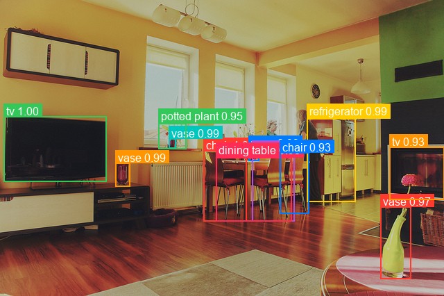
Label text is drawn just above each box and clamped to stay on-canvas, so a detection touching the top edge keeps its label visible.

plot_segmentation

plot_segmentation(image, segmentation, class_names=None, ax=None, alpha=0.55,
                  cmap="tab20", show_legend=True, legend_top_k=8, title=None,
                  figsize=(10, 7), seed=42)

Overlays a (H, W) integer label map on the image. Semantic, instance, and panoptic all work, since all three come back as an id map.

Parameters

• segmentation: (H, W) integer array of class or instance ids.
• class_names (optional): list indexed by label id. Without it the legend reads class_12.
• alpha (defaults to 0.55): overlay opacity.
• cmap (defaults to "tab20"): used when the label space fits the colormap.
• show_legend / legend_top_k: legend of the largest segments by pixel area, capped at 8.
• seed: palette seed for large label spaces.

from kerasformers.utils import plot_segmentation
from kerasformers.utils.labels_util import ADE20K_150_CLASSES

seg = processor.post_process_semantic_segmentation(outputs, target_size=(h, w))
plot_segmentation(image, seg["segmentation"], ADE20K_150_CLASSES)

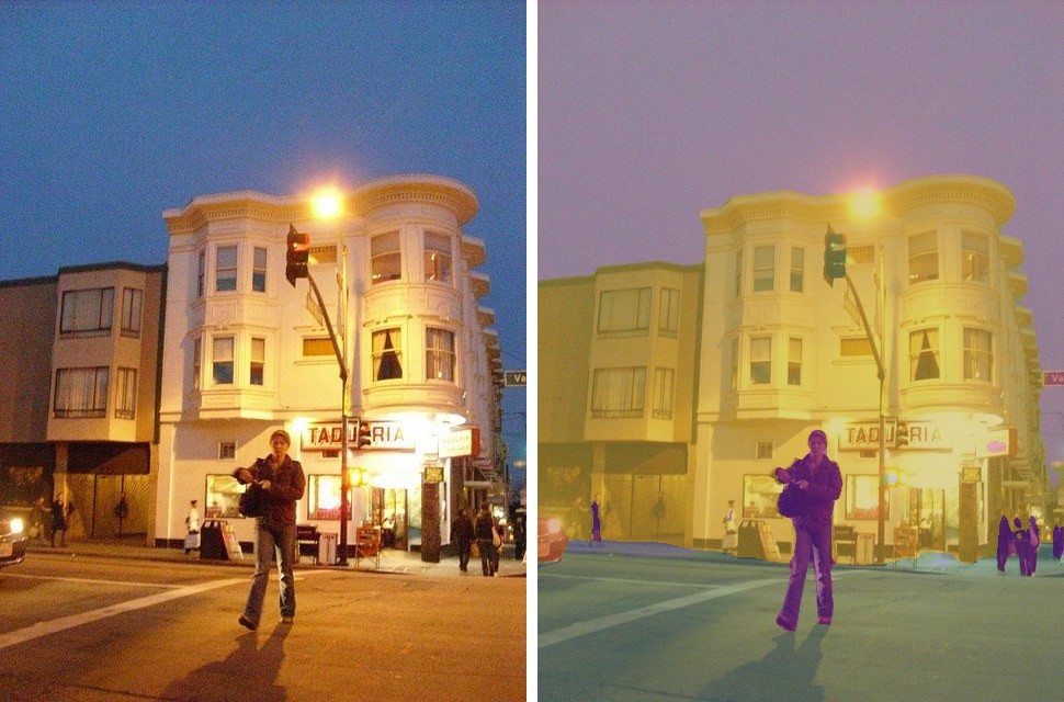
Two behaviors worth knowing. Above 20 labels tab20 runs out, so a deterministic random palette takes over, keyed on seed: the same scene colors identically across runs, but the colors are not the dataset's canonical ones. And negative ids are treated as background, left showing the source image, which is what makes EoMT's "no class" regions render sensibly rather than as a class 0 blanket.

plot_depth

plot_depth(image, depth, side_by_side=True, cmap="inferno", ax=None, alpha=0.55,
           title=None, figsize=(12, 6))

Image and depth map side by side, or overlaid when side_by_side=False.

from kerasformers.utils import plot_depth

depth = processor.post_process_depth_estimation(outputs, target_sizes=[(h, w)])[0]
plot_depth(image, depth["predicted_depth"])

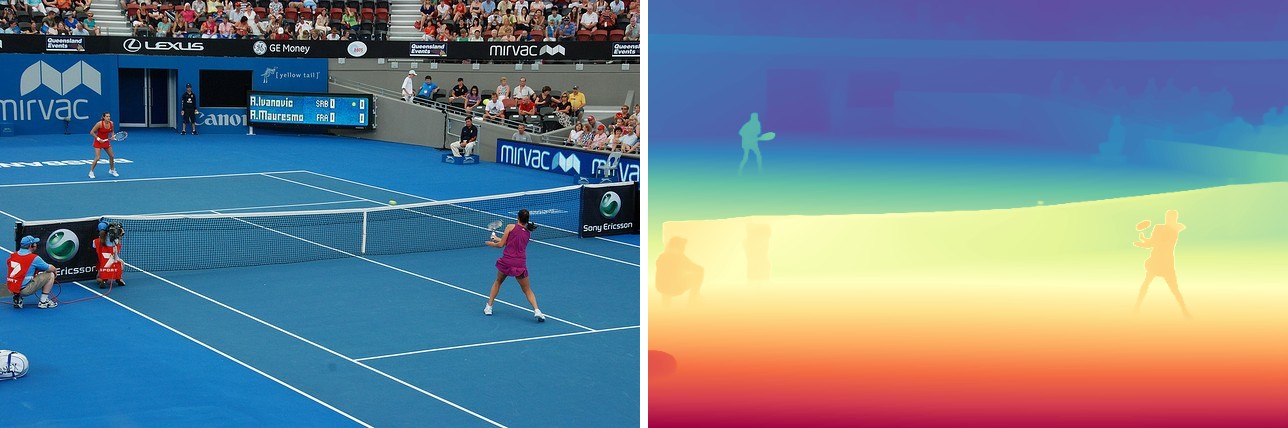
Depth is min-max normalized per image before coloring. Relative-depth models produce values on an arbitrary scale, so this is the only way to get a usable picture, but it means colors are not comparable between two figures: the same shade in two plots can be very different distances. For metric models, plot the raw values yourself if absolute scale is the point.

This is the one helper that does not always return an axis: with side_by_side=True it creates two, so it returns (fig, axes). Overlaid, it returns the single axis.

plot_sam_masks

plot_sam_masks(image, masks, scores=None, points=None, point_labels=None,
               boxes=None, ax=None, alpha=0.55, colors=None, title=None,
               figsize=(10, 7))

Binary masks plus, optionally, the prompts that produced them, so you can see where you clicked and what came back. Covers SAM, SAM 2, and SAM 3.

Parameters

• masks: (N, H, W) or (H, W) binary masks, already thresholded.
• scores (optional): per-mask IoU predictions.
• points / point_labels (optional): (N, 2) xy prompts; label 1 draws green (foreground), 0 draws red (background).
• boxes (optional): box prompts, drawn alongside.
• colors (optional): per-mask colors, otherwise tab20 cycled.

from kerasformers.utils import plot_sam_masks

plot_sam_masks(image, masks[0], scores=scores[0],
               points=input_points, point_labels=input_labels)

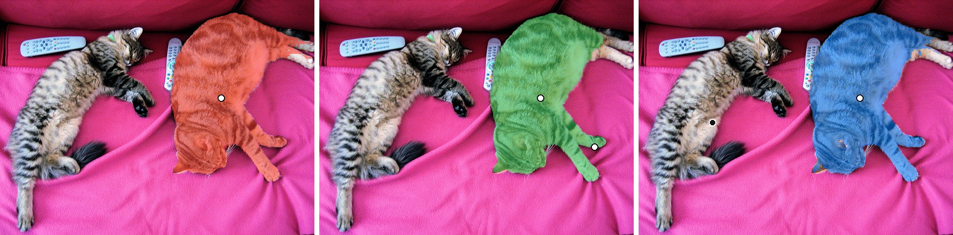
Pass raw logits and you get a full-frame mask, since every pixel above 0 counts as active. Threshold first.

Building your own

The four helpers above are compositions of smaller pieces, all importable from kerasformers.utils.visualization_util:

Helper	Does
get_axes(ax, figsize)	Return ax, or create a figure when it is None. The reason every helper accepts ax=None.
to_numpy(x)	Convert any backend tensor to NumPy, passing None through.
plot_image(image, ax, title, figsize)	imshow with the axes hidden.
plot_boxes(boxes, labels, scores, ...)	xyxy rectangles with label text.
plot_masks(masks, ax, colors, alpha)	RGBA overlays for (N, H, W) masks.
plot_points(points, labels, ax, ...)	Foreground/background prompt markers.
overlay_depth(depth, cmap, ax, ...)	Min-max normalized depth, no background image.

Composing them is how you get a figure the wrappers do not cover, for example boxes and masks together on one axis:

import matplotlib.pyplot as plt
from kerasformers.utils.visualization_util import plot_image, plot_masks, plot_boxes

fig, ax = plt.subplots(figsize=(10, 7))
plot_image(image, ax=ax)
plot_masks(masks, ax=ax, alpha=0.5)
plot_boxes(boxes, labels=names, ax=ax, color="yellow")
plt.savefig("combined.jpg", bbox_inches="tight", dpi=150)

Note that only the four top-level functions are in __all__; the pieces are reached through the module path.

See also Image utils, Video utils, and Class labels.